
Collider bias (extended version)
Bias may be inadvertently introduced to a drug effect study by restricting the study sample or controlling for a variable that is a “collider”.

In the general population, height and speed are not strongly correlated. Knowing someone’s height tells you little about how fast they are.
Now imagine a team of NBA players. You notice a 5’8” player who is blazingly fast and agile. Suddenly, height becomes informative. Why? Because only the most exceptional short players make it into the NBA, usually by being much faster, more agile, or more skilled than their taller peers. Meanwhile, taller players can "afford" to be slower and still get selected due to their size advantage.
The figure below shows this:
The grey dots represent individuals in the general population (height vs. speed).
The orange dots represent NBA players, a selected subset.
If you fit a line to the orange dots, it would show a negative (inverse) relationship between height and speed. Among NBA players, the shorter you are, the faster you probably are, and vice versa.
This is a classic case of selection bias (or collider bias) introduced by conditioning on being in the NBA, a variable influenced by both height and speed. The act of selecting on this common effect (NBA membership) induces a spurious correlation between two variables that are otherwise unrelated in the general population.

If our target population for our scientific question is the general population then restricting the study population to the NBA players creates a spurious association between height and speed. In other words, if one conditions or restricts to NBA players, this induces bias. This particular type of bias is known as collider bias.
Defining Collider Bias
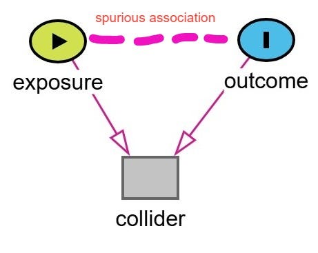
Collider bias is a subtype of selection bias that occurs when we condition on a variable that is a common effect (a collider) of two other variables. This conditioning, whether through regression adjustment, stratification, or restriction, can induce a spurious association between those variables, even if no causal relationship exists between them.
Key features of collider bias:
the distortion can range from small to large
it can lead to overestimation or underestimation of a treatment effect
it can even reverse the direction of an observed assocation
Causal diagrams or DAGs (direct acyclic graphs) are one of the best tools for identifying potential colliders. They help clarify whether a variable should be adjusted for, or avoided, in order to preserve the validity of a study’s findings.
Examples of Collider Bias in the Health Sciences
The NBA example is fun but let’s move on to some more topical examples in the health sciences.
A classic form of collider bias is known as Berkson’s bias, also referred to as Berkson’s paradox, or Berksonian bias.1 It arises when hospitalization is the collider.
This bias occurs when a study is restricted to a hospital-based sample, and two variables that each increase the likelihood of hospitalization, such as a disease and a risk factor, become spuriously associated through conditioning on the collider.
This can lead to a false inverse association between the two variables. In other words, it might look like the risk factor is protective against the disease—when in fact it's not. This is the classic scenario often cited in Berkson’s original work. However, it's important to note that Berkson’s bias does not always result in a negative or inverse association. Depending on the structure of the relationships, it can can create a spurious positive association, mask a true association, or reverse the direction of a true association.
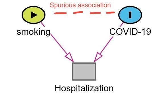
Berkson’s bias was a real concern in early COVID-19 research.2 One widely cited example is the spurious protective association between smoking and the incidence of COVID-19 or COVID-19 severity.3
Lets walk through how this bias emerges. In this example, shown below in the figure, hospitalization is the collider (common effect of both COVID-19 severity and smoking status). Patients with more severe COVID-19 symptoms are more likely to be hospitalized. Patients who smoke are admitted to the hospital for a variety of conditions associated with smoking irrespective of their COVID-19 status. As a result, among hospitalized patients smokers with mild or moderate COVID-19 may be overrepresented as the reason for admission was related another condition related to their smoking status (ie. COPD, cancer, heart disease). Non-smokers are more likely to be hospitalized only if their COVID-19 symptoms were severe. Therefore, in a study restricted to hospitalized patients, it may appear that smokers are less likely to have severe COVID-19 or COVID-19 at all. This is a spurious association created by conditioning on hospitalization (the collider).
The previous diagram forms a classic “V-shaped” structure, often used to illustrate collider bias. There are several other DAG “shapes” that can also signal the presence of collider bias.
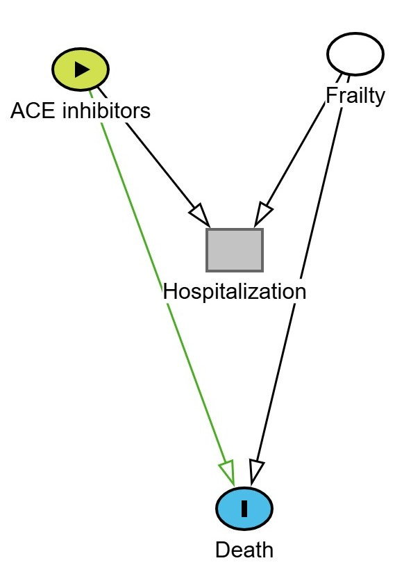
A “Y” type shaped diagram can illustrate how collider bias arises when a risk factor for the outcome shares a common effect with the exposure. An example of this is shown below where ACE inhibitors (exposure) and frailty both increase the likelihood of hospitalization. Hospitalization is the collider. Frailty also increases the risk of death (the outcome).
If we restrict the analysis to only hospitalized patients, we are conditioning on a collider (i.e. hospitalization). This opens a backdoor path between ACE inhibitors and frailty, and since frailty affects death, we may induce a spurious association between ACE inhibitor use and death, even if no true causal link exists.
This is depicted in the DAG below. The green line represents the biased (non-causal) path that becomes active when conditioning on hospitalization.
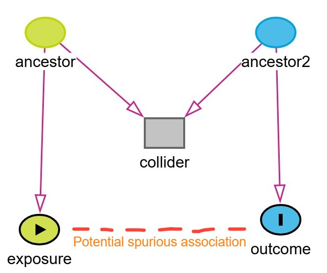
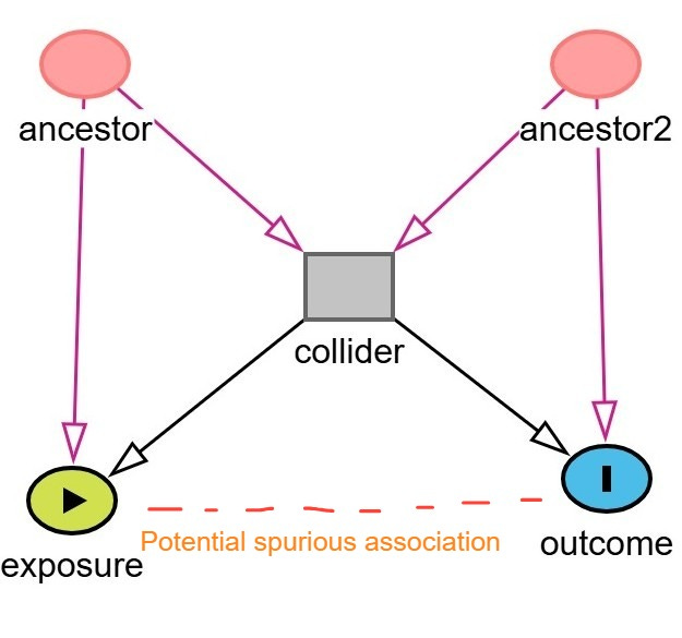
A more complex subtype of collider bias is known as M-bias (or M-type collider bias). This occurs when one conditions on a variable connected by two otherwise unconnected paths, thereby forming an “M” shape in a DAG. In M-bias, the ancestors of both the exposure and the outcome influence a shared collider, and conditioning on this collider induces a spurious association between the exposure and the outcome, even though no true causal path exists between them.
An example of M-bias is shown below. In this example, the exposure is coffee and outcome is heart disease. Stress (ancestor / unmeasured variable) is a cause of increased coffee consumption. Diet (Ancestor2 / unmeasured variable) is a cause of heart disease. Sleep quality is a collider influenced by both stress and diet. If we condition on sleep quality, by adjusting for it in regression or stratifying the analysis, we may inadvertently induce an association between coffee consumption and heart disease through the non-causal backdoor path:
Coffee ← Stress → Sleep Quality ← Diet → Heart Disease
Thus, a biased connection is introduced between the exposure and the outcome through their respective ancestors and the shared collider.
A even more complex subtype of collider bias is known as butterfly bias. It’s a double whammy, a lose-lose situation! Let’s return to the the example above whereby coffee is the exposure, heart disease is the outcome, and sleep quality is the collider. The unmeasured variables, stress and diet both influence sleep quality and are ancestors of coffee and heart disease. Now, let’s assume sleep quality also directly affects both coffee consumption and heart disease, making it a confounder as well.
This creates a butterfly-shaped structure in the DAG where sleep quality sits in the middle of paths acting both as a collider and a confounder. Conditioning on sleep quality may help adjust for confounding, but it also opens a backdoor path via the collider structure, inducing bias. In this scenario, you're stuck with a trade-off:
Adjusting for sleep quality controls confounding but risks collider bias.
Not adjusting avoids collider bias but leaves residual confounding.
It’s a true "lesser of two evils" situation—highlighting why causal diagrams (DAGs) are essential for deciding what to adjust for.
Collider Bias in Randomized Controlled Trials
Collider bias can even occur in an RCT especially when there is differential loss to follow-up between treatment arms.
Imagine a trial that randomizes 500 patients in a 1:1 manner (with proper allocation concealment) to either treatment or control. Now suppose 15% of patients in the treatment arm and 30% in the control group are lost to follow-up. Further, assume that patients with an unmeasured variable, such as greater severe disease, poor adherence, or more adverse effects are more likely to drop out.
If the unmeasured variable also affects the outcome, and we restrict the analysis to patients who remained in the study, we are effectively conditioning on a collider (i.e.. loss to follow-up).
This can open a non-causal path between treatment and outcome through the unmeasured variable, introducing collider bias. The result? A biased estimate of the treatment effect—even in an intention-to-treat framework if the analysis includes only complete cases.
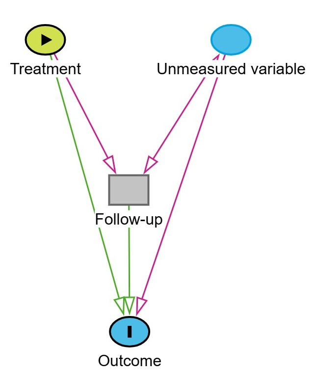
This scenario is represented by a “Y-shaped” DAG, where:
Treatment and the unmeasured variable both affect follow-up (the collider),
And the unmeasured variable also affects the outcome.
If you are looking for more examples of collider bias, check out the paper by Digitale and colleagues published in the Journal of Clinical Epidemiology.4
Avoiding Collider Bias
Collider bias is best avoided by thoughtful study design.5 One key principle is to avoid restricting the study population based on variables that are affected by both the exposure and the outcome. For example, limiting inclusion to individuals who experience a post-exposure event (like hospitalization) can introduce bias if that event is a collider.
Other strategies include:
Minimizing loss to follow-up, especially when dropout is influenced by both treatment and outcome-related factors.
Drawing a DAG (directed acyclic graph) during the study planning phase, which can help identify potential colliders and inform decisions about which variables to adjust for—or avoid adjusting for—in the analysis.
Designing your analysis plan to avoid conditioning on colliders through methods such as multivariable regression or stratification.
Putting It in Context
Epidemiologists typically classify threats to internal validity into three main categories: selection bias, information bias, and confounding. Collider bias falls under selection bias.6 It can arise through:
Selection into a study, such as sampling only hospitalized patients, and/or
Selection out of a study, such as through differential loss to follow-up or missing data.
Being aware of these pathways during both design and analysis is essential for drawing valid causal inferences.

